SWITCH Function
A Logical Function in Excel that compares a given value against a list of values and returns the result for the first matching value from the list.


What is the SWITCH Function?
The SWITCH function is a Logical Function in Excel that compares a given value against a list of values and returns the result for the first matching value from the list.
Why do you think the function is named so? It does nothing like turning a light bulb on or off. So what does Excel intend to tell you?
We believe that the meaning behind the function's name is in its ability. The function can 'switch' through the values in the list if a suitable match isn't found.
If no match is found, the user can ultimately return a default value from the given list. The function sounds impressive so far, but it has been one of the most overlooked functions because many people have been unable to understand what it does or how it works.
We won't just be singing praise for the function since it undoubtedly has its drawbacks.
In this article, we will learn the function's syntax, how to use it, and a couple of examples.
Key Takeaways
- The SWITCH function is a Logical Function in Excel that is used to evaluate an expression against a list of values and return a corresponding result.
- Users provide an expression to evaluate and a series of value-result pairs. It returns the result corresponding to the first matching value.
- Users might encounter potential errors when using the SWITCH function, such as providing invalid input values, referencing cells with incorrect data, and not knowing how to address them effectively.
- SWITCH function finds applications in data analysis, report generation, and data transformation tasks, where conditional value selection is essential for manipulating and summarizing data based on specific criteria.
Understanding the SWITCH function
The SWITCH is a logical function that evaluates a value to all the values in the list and returns the result for the first match found.
For example, suppose that our value is 'money.' Then, the list, along with its corresponding values, is illustrated below:
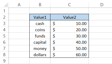
If 'money' exists in our list, the function would be able to return the corresponding result from the 'Value2' column.
As you can see, the value exists in cell B7 so that the function can extract $50.00 from column' Value2.'
The function was introduced in Excel 2016 and was not available in previous versions. However, the function was earlier available in VBA.
If you are tired of using the complex nested IF formulas, then you can use the SWITCH function as its substitute. The function works on a similar principle and returns the result based on the first match it finds.
SWITCH Function Formula
The Excel community has overlooked the function not because it is challenging to use but because we have either been unaware of its capabilities or entirely overdependent on its alternatives.
Perhaps understanding the syntax for the function will prove this to us.
The syntax for the function is:
=SWITCH(expression,value1,result1,[default_or_value2,result2],...)
where,
- expression - (required) the value that we want to compare. There are no rules when you input the argument, i.e., it can be a numerical value, date, time, or even a text string.
- value1 - (required) the first value against which the expression argument will be compared
- result1 - (required) the corresponding value that the function would return if the match is found.
- default - (optional) value that is returned if the expression does find a match to any values on the list.
- value2 - (optional) the second value against which the expression argument will be compared
- result2 - (optional) the corresponding value that the function would return if the match is found.
Note
You can input 126 pairs of values and results while using the function.

How to use the SWITCH Function in Excel?
Like most of our Excel articles, this section won't be an exception. Here too, you can utilize two different methods to use the function.
They are:
Method 1: From the function's library
A function is a predefined formula that takes arguments in text boxes and returns our result in the selected cell.
The only complaint most Excel users have with this method is that it does not offer greater flexibility. To select the function, please follow the steps below:
1. First, select the cell in which you intend to return the result.

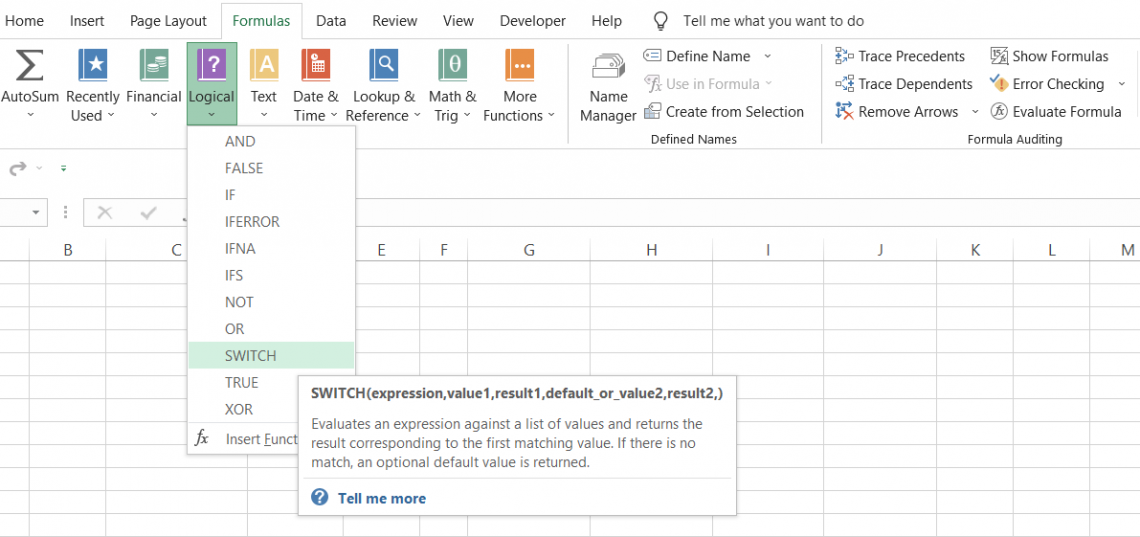
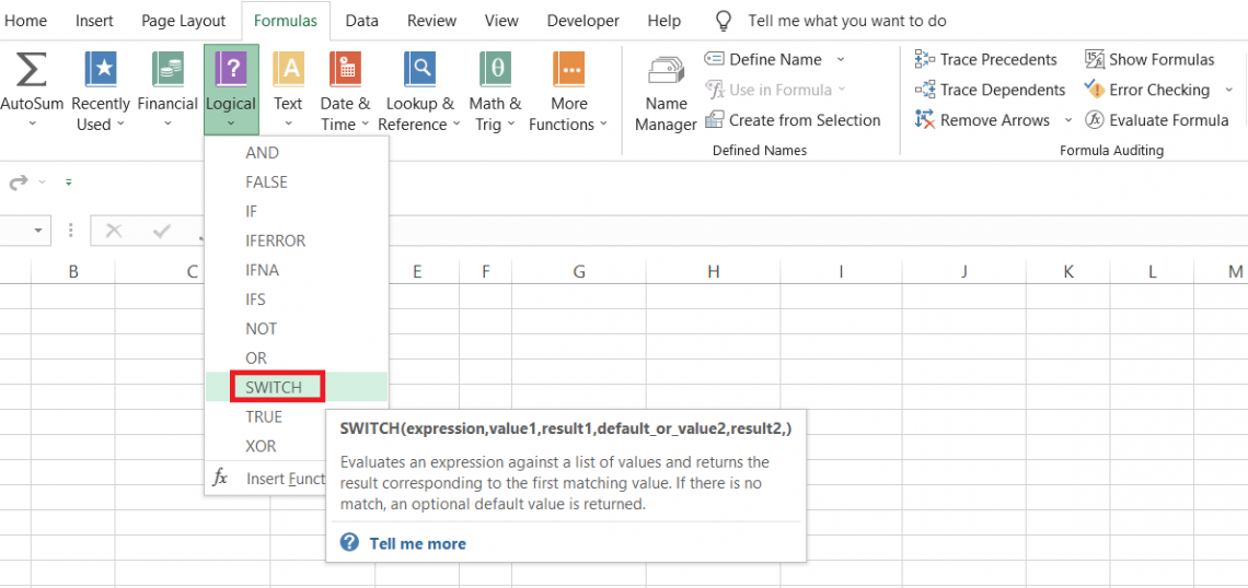
2. Click on the Formulas tab > Logical > and select the SWITCH function.
3. This will open up the dialog box as illustrated below:
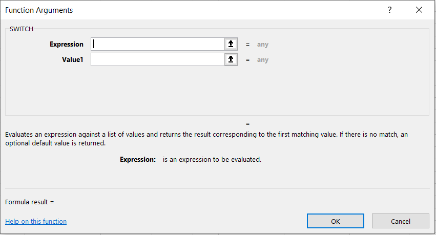
4. Suppose the value in cell B2 was 'money.' We will reference the cell of Expression argument while the rest of the arguments are as illustrated below:
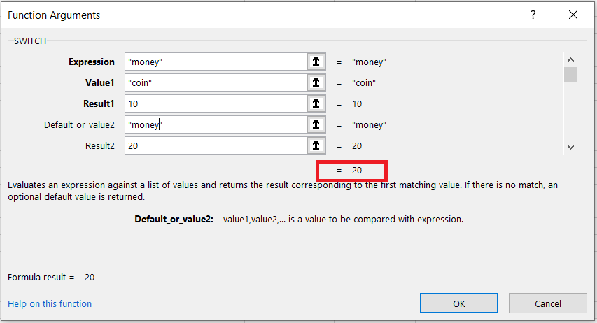
5. You do get a preview of the result in the dialog box itself. As you can see, we get a result of 20. If there were no matches, we would get a preview of 'no value found.'
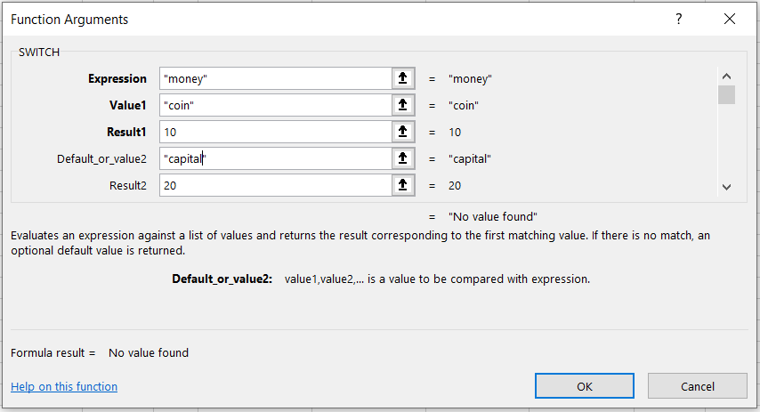
The function doesn't return an error if the value is not found. So you can customize the default text. However, if you ignore it, the function will return the text 'No value found'.
Method 2: As a worksheet formula
Most users in the Excel community prefer using the functions as a worksheet formula. It saves loads of time, offers more flexibility, and helps incorporate many functions together.
All you need to do is begin with an equal sign(=), type in the function name, and input the arguments per the function's syntax.
Suppose that you have the data as illustrated below:
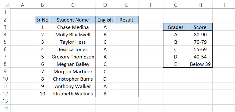
The corresponding test scores based on the grades lie in column H. Based on the data available, the formula will be
=SWITCH(D3,$G$4,$H$4,$G$5,$H$5,$G$6,$H$6,$G$7,$H$7,$G$8,$H$8)
The formula gives us the result:
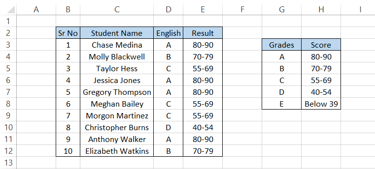
The function evaluates the cell in column D and compares it against the column G values. If there is a match, the value in the next column, i.e., column H, returns as our result.
As we said earlier, SWITCH is a simplified version of nested IF. For example, if you use the IF function, then the formula would be =IF(D3=$H$4,$I$4,IF(D3=$H$5,$I$5,IF(D3=$H$6,$I$6,IF(D3=$H$7,$I$7,IF(D3=$H$8,$I$8))))), giving you a similar result as:
There are times even when great Excel wizards cannot decode such complicated nested IF formulas.
SWITCH is not only easier to understand but to write as well. However, we would still recommend studying both functions as each has advantages!
SWITCH Function Example
Here comes the most awaited part - some practical examples! If you see some situation where you are using multiple IF statements, you can easily substitute it with the SWITCH function.
Example 1
You might have noticed that the SWITCH function returns results with exact matching values. As for the previous example, we saw that the score range was returned when we input the 'specific' grades as our expression.
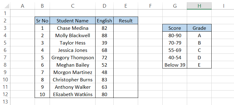
But what if we did not have grades in the data and instead those were test scores?
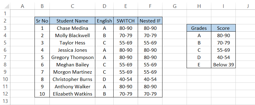
Suppose the data looks as illustrated below:
Based on the test scores in English, we can derive the grades using the formula =SWITCH(TRUE,D3>=80,"A",D3>=70,"B",D3>=55,"C",D3>=40,"D","E") which gives the result:
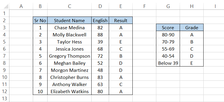
Hmm, let's check whether the results are accurate. Chase scored 82, which is graded A; Anthony's score falls within the 55-69 range, so it's a C. Looks all good!
So what went behind the scenes? Let's break down the formula to understand it better.
- We set up our expression as a boolean value TRUE.
- Next, we use the comparison operators to compare the cell value in column D with our ranges in column G (we have hardcoded the values instead of referencing them).
- Whichever of these comparisons first evaluates to TRUE, i.e., equal to our expression, we get the corresponding value in column E.
- For example, Meghan Bailey scored 52 on her English Test. Our first logical statement is D3>=80, which is false, allowing us to move on to the following logical statement, which is D3>=70.
- Our fourth logical statement, i.e., D3>=40, meets the criteria, evaluates to TRUE, matches our expression statement, and returns the result as 'D.'
- If none of the logical statements had matched, our default value was 'E.' These grades represent all the test scores equal to or below 39. For example, Taylor Hess scored 39 on the English Test and received an E.
Example 2
Let's see another similar example. Suppose that the company makes purchases on the following dates as illustrated below:
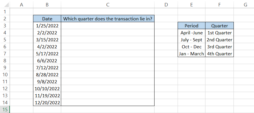
It would help if you determined in which quarter the purchases were made so that it's easier to group the data.
Here, we will use the formula =SWITCH(TRUE,MONTH(B3)>=10,"3rd Quarter",MONTH(B3)>=7,"2nd Quarter",MONTH(B3)>=4,"1st Quarter",MONTH(B3)>=1,"4th Quarter") and drag it down up to the cell C14, which gives us the result:
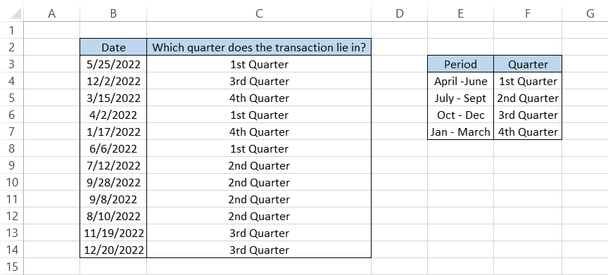
Again, a similar logic follows in our example. When the logical statement returns as TRUE, it matches our expression. Then the corresponding value, i.e., the quarter in which the transaction was done, returns in the spreadsheet.
However, did you wonder why we began with MONTH(B3)>=10 in the formula rather than MONTH(B3)>=1?
The logic is straightforward. SWITCH returns the result for the first match it finds amongst our inputs. The MONTH function returns the month value from the given date. Since all the months are more significant than 1, we would have ultimately got all the results as '1st Quarter'.
To avoid these conflicting results, always ensure that you compare the most significant value first using the logical operators and go towards the lowest number along the way, i.e., MONTH(B3)>=1
This way, the integrity of the sequence is maintained, and you will get the correct results.

SWITCH vs. NESTED IF
The SWITCH function was introduced as an alternative to finding the first TRUE value for exact matches. The nested IF statements were previously the go-to tool for most excel users in case of finding the first TRUE value for exact matches. However, they were a bit difficult to interpret.
When you have too many inputs, there is a high probability you might get lost as to what arguments you still need to input.
The syntax for the IF function is:
=IF(logical_test,[value_if_true],[value_if_false])
where,
- logical_test = the condition that you want to test
- value_if_true = the value that is returned by the function if the condition evaluates to TRUE
- value_if_false = the value that is returned by the function if the condition evaluates to FALSE
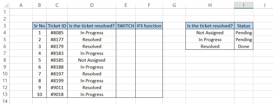
Suppose an IT support company tracks its ticket systems through Excel. The ticket status would be displayed as 'Pending' or 'Done' based on the values in column D.
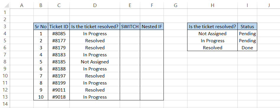
When the ticket is either 'In Progress' or 'Not Assigned,' the status is 'Pending,' while for 'Resolved,' the status is 'Done.'
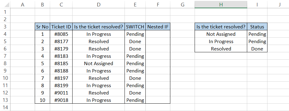
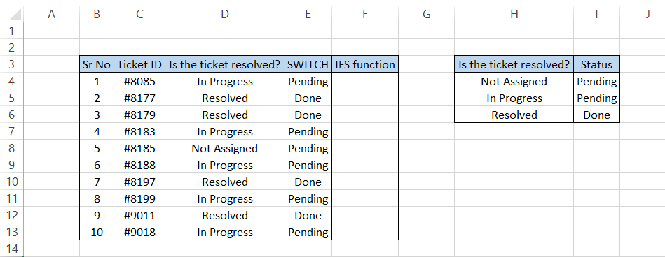
Using the SWITCH function, the formula in cell E4 would be =SWITCH(D4, "Not Assigned", "Pending", "In Progress", "Pending", "Resolved", "Done") which you can drag up to the cell E13 to give the result:
Similarly, the IF functions can be nested to get a similar result. The formula will be =IF(D4="Not Assigned","Pending",IF(D4="In Progress","Pending",IF(D4="Resolved","Done"))) which gives the result:
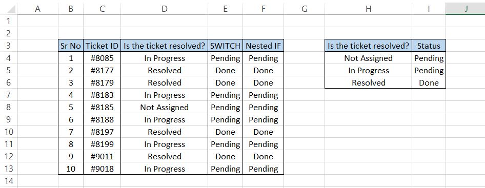
The secret behind the Nested IF statements is that whenever the formula evaluates to FALSE, we input another IF statement that runs to check if the condition is TRUE. The formula continues until we find that particular value or get the result as FALSE or a customized text string.
SWITCH vs. IFS
The IFS function, introduced in 2016 as an alternative to nested IF statements, works similarly to the nested IF and SWITCH functions.
The function allows us to input multiple conditions and returns a value based on the first TRUE match.
The syntax for the IFS function is:
=IFS(logical_test1,value_if_true1,[logical_test2],[value_if_true2])
where,
- logical_test1 - (required) The first condition that you want to evaluate
- value_if_true1 - (required) The value that is returned when the condition evaluates to TRUE
- logical_test2 - (optional) The second condition that you want to evaluate
- value_if_true2 - (optional) The value that is returned when the condition evaluates to TRUE.
Note
You can use 126 optional logical statements/value_if_true pair in this function that evaluates to TRUE or FALSE.
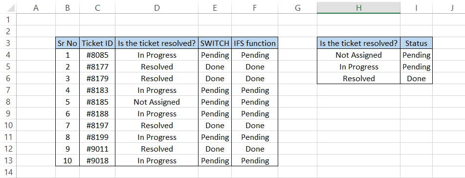
Returning to our example of a ticket tracking spreadsheet for the IT support team, the data looks as illustrated below:
The formula in cell E3 would be =SWITCH(D4,"Not Assigned","Pending","In Progress","Pending","Resolved","Done") which you can drag up to the last cell to get the result:
On other hand, to find the result using the IFS function, the formula will be =IFS(D4="Not Assigned","Pending",D4="In Progress","Pending",D4="Resolved","Done"), which gives the result:
See? The same results while the formula is not that different too. The question arises: Why did Excel go to such lengths to have functions with similar capabilities?
SWITCH function primarily allows you to test only one logical condition, whereas the IFS function will allow you to input multiple conditions.
Yes, you can input more than one logical condition in SWITCH, as we saw in one of the examples in the function where we incorporated the TRUE function. Whatever condition matched with TRUE, we got the corresponding result.
However, the point is that if you want to compare just one value for its exactness, then SWITCH should be your go-to tool.
Free Resources
To continue learning and advancing your career, check out these additional helpful WSO resources:
or Want to Sign up with your social account?