ROWS Function
Provide the number of rows within a reference or an array.


What is the ROWS Function?
Rows is a function in Excel designed to provide the number of rows within a reference or an array. This tool counts the number of rows within a specific range. It is labeled as a Lookup and Reference function.
This function would be of great use to us if we wanted to find out how many rows there are between one referenced cell to another. This function is helpful for anyone, from students to employees, employers, and people wanting to know more about Excel.
The syntax for this function is
=ROWS(array)
where
array = the reference to the range of cells you chose to select.
We will explain how this formula works in greater context by providing examples. This is a straightforward calculation. First, select the cells you want to reference for your array, which should return the number of rows within that specified range.
NOTE
Rows will only return the number of rows no matter which columns are selected or if you selected one line across columns.
Key Takeaways
- The rows function calculates the number of horizontal lines mentioned in Excel and returns the value in an array.
- It is helpful for anyone, whether you’re an employer, an employee, a student, a teacher, or someone who uses Excel for fun or in their off-time.
- If the cells you chose have numeric values, the function will still return the number of lines you’ve chosen, no matter what’s in the cells.
- Rows and Row functions differ from one another. The Row feature returns the row number that’s being referenced. If you select more than one row, you get back more than one answer.
- You can use addition, multiplication, subtraction, and addition with Rows. For instance, if you select cells J4 through J8 and divide by 2, you get an answer of 2.5. The reason is that there are 5 lines, and you’re dividing by 2, so your answer is 2.5.
Example of ROWS Function
ROWS function is a straightforward tool to use. All you have to do is insert the syntax [=ROWS()] and select the cells you want to be referenced and you should get the number of rows back from those referenced cells.

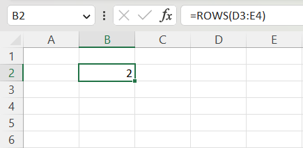
Let’s use D3:E4 for our array.
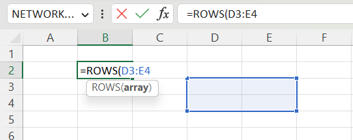
Once we’ve put D3:E4 in the parentheses, we got 2 as the answer as only 2 rows were referenced here (lines 2 & 3).
We’ll go over this in greater detail with more examples. Below is a screenshot of the examples using this function.
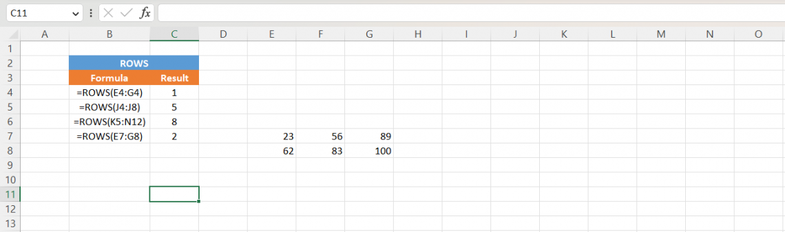
As you can see above, this function shows how many rows we’ve referenced. In our first example, using =ROWS(array) with cells E4 through G4 as our array, we got an answer of 1 because only one row is referenced.
Next, you want to find out what the answer would be if only one column were chosen. Using column J with cells J4 through J8 being selected for our array, we got a solution of 5 rows.
Then, suppose you want to figure out what the answer will be if you select multiple columns. Using cells K5 through N12 as our array, we got a solution of 8 as only eight lines are being referenced.
Finally, you want to know if this function works on cells with numeric values. Using cells E7 through G8 as our array, we got an answer of 2 because this function only returns the number of rows referenced regardless of any numeric values in them.
ROWS vs. ROW Function
Now that we have a pretty good idea of what ROWS does, you may wonder what row is.

The Row function returns the row number from a referenced cell. In addition, it returns the referenced number of the specified cell(s).
The syntax for this function is
=ROW([reference])
where
reference = the number of the referenced row.
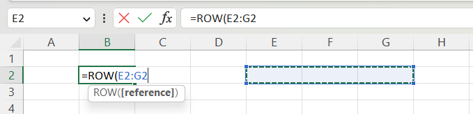
The ROW function is easy to use. You have to input the syntax above, select the number of cells you want to choose, and you should get back the row number from those cells. For example, let’s use cells E2:G2 as a reference point.
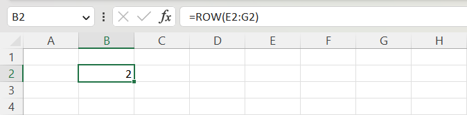
Now that we imputed E2:G2 for the reference, we got 2 back as our answer because all the chosen references are in the 2nd row.
We will use this formula in greater context by providing examples and looking at how Rows and Rows differ. Below is a screenshot using the same problems from the last screenshot and new examples using the row feature.
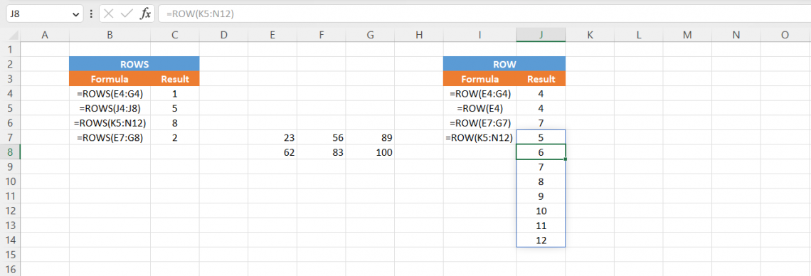
As you can see from the first example, Rows give us the number of horizontal lines being referenced, while row provides us with the row number.
Using =ROW([reference]) and cells E4 through G4 as our reference gave us an answer of 4 because only the 4th row is mentioned.
Next, you wanted to determine what would happen if you chose only one cell. Using the same method we used to calculate our first example, with E4 being our selected cell, we still got an answer of 4 as it only returned the row number.
Then, you wanted to see what would happen if you selected cells with numeric values. Again, using E7 through G7 as our example, we got an answer of 7, meaning that our row number is still 7, no matter if there are numeric values within a specified range of cells.
Finally, you wanted to know what would happen if you selected multiple lines. Again, using cells K5 through N12 as our reference, we got back more than one answer; we got 8 different numbers because we selected more than one row.


or Want to Sign up with your social account?