IFS Function

What is the IFS Function?

Imagine you need to rapidly organize a stack of documents with various responsibilities and due dates.

Using the IFS function in Excel is like having a personal assistant who can quickly evaluate each task and tell you which is the most urgent based on your established rules.

It is a feature launched with Microsoft Excel 2016 as a user-convenient alternative to NESTED IF, which was a bit inflexible and difficult to use under multiple conditions.

The function is useful when dealing with multiple problems at once and having to make complex decisions. This helps evaluate many conditions efficiently and provides a flexible way to manage the task.

Syntax of IFS Function

The function has a pretty simple syntax. The opening parenthesis, the function name, the conditions, and their values are listed in the order given in the formula.

The function offers great versatility in tackling challenging data analysis jobs since it allows the evaluation of up to 127 criteria.

The function's syntax is far less complex and convoluted than nested IF statements, which lowers the risk of mistakes.

Syntax

IFS(logical_test1, value_if_true1, [logical_test2, value_if_true2], [logical_test3; ...)

Where:

1. Condition1, Condition2…Condition_n = The condition we wish to test. It could be a value, an expression, or a reference to a cell that already has one. Any logical argument that yields TRUE or FALSE is acceptable here.
2. Value1, Value2…Value_n = The values that respect the tested conditions and are returned corresponding to them being TRUE.

Each pair of condition and value_if_true is separated by a comma. The function evaluates the conditions in the order they are provided and returns the value corresponding to the first condition that evaluates to TRUE. If none of the conditions are met, the function returns the #N/A error.

How to use the IFS function

It's a built-in, powerful tool in Excel for testing multiple conditions and returning the first value that corresponds to be true.

This function allows you to create more complex calculations in Excel, as it can test up to 127 different conditions.

Excel's IFS function is a helpful tool for managing intricate circumstances. You may simplify and improve the efficiency of your calculations by utilizing this function.

You may develop more intricate and potent spreadsheets by skillfully using the IFS feature with practice.

The steps to use the function are as follows:

1. Enter the IFs function in the cell
Decide the cell where the function has to be input. Then, type the equal sign (‘=’) to begin the function, followed by ‘IFS(’ in the search box to access the function.

2. Write the initial logical argument
When you enter the function, the symbol =IFS( appears in your chosen cell. Then, below the open parenthesis, enter the first logical test you wish the function to run.

To initiate the test, you will have to enter certain operators. There are two types of operators used in MS Excel:

A. Comparison Operators 

These operators let you compare two values and return a logical value based on the result of the comparison, whether true or false.

The following comparison operators are acceptable for your logical tests:

• Less than (<)
• Greater than (>)
• Equal to (=)
• Not equal to (<>)
• Less than or equal to (<=)
• Greater than or equal to (>=)

B. Logical operators 

These operators allow you to combine two or more logical values and return the resulting logical value. The following logical operators are available in this function:

• AND: If all arguments are TRUE, this function returns TRUE.
• OR: This runs the argument and returns TRUE even if one of them is TRUE.
• NOT: This function returns the inverse of the argument (TRUE becomes FALSE, and vice versa).

3. Enter the first argument

After your first logical test, use a comma and put the value you wish to appear if the condition is met. For example, if you want a number as the value, enter a number followed by a comma.

For example: If you want Excel to return a grade ‘A’ if the marks of a student are above 90, then the function would look like this-

=IFS(A1>90, “A”, )

4. Enter more logical arguments to test

The IFS function just needs one logical test and a value if it is true, but you can add more by repeating steps two and three. Ensure to separate each logical test and value with a comma.

When you're finished, add a closing parenthesis to the end of the final value if it's true.

For example:

=IFS(A1>=90,"A",A1>=80,"B",A1>=70,"C",A1>=60,"D",A1<60,"F")

The first condition instructs the function to return "A" if A1 is greater than 90. If A1 is less than 90, the function runs the other tests until it finds a true condition. For example, if A1 includes 82, the function will return "B."

Examples of IFS function in Excel

When working with data in Excel, the IFS function can be a helpful tool for categorizing and evaluating data depending on various conditions.

The IFS function can help you speed up your data analysis and make more informed decisions by allowing you to assess numerous criteria at once.

In the following examples, we will look at various ways to use the IFS function in Excel, from simple grading systems to more intricate spending categorizations.

Example 1 

Assume a teacher has 10 students under his apprenticeship. The students are studying 5 subjects, and he decides to test them on the subjects.

Post the assessment, they’re awarded the following marks:

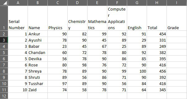
The teacher maintains an Excel sheet for the students to keep things handy with neatness and precision. He later has to grade the students based on their overall performance to understand their learning throughout the semester better.

The formula user here will be

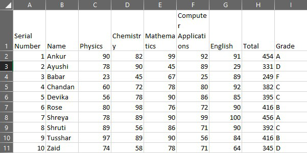
=IFS(H2>450,"A",H2>400,"B",H2>350,"C",H2>300,"D",H2<300,"F")

The formula depicts various parameters for deciding the students' grades.

One who scored above 450 is allotted a grade ‘A,’ one above 400 but below 450 a grade ‘B,’ likewise above 350 a grade ‘C,’ the one above 300 and below 350 a grade ‘D,’ and one who has scored below 300 a grade ‘F.’

After copying the formula in column ‘I,’ the spreadsheet would yield the following result:

Remember, IFS is a conditional statement, i.e., it evaluates the logical tests provided and returns the prescribed value accordingly.

It runs a loop and returns the value according to the conditions given. If all requirements are false, the IFS function does not return a value.

Therefore we put an ‘H2<300’ at the end of the function so that if none of them are triggered to deliver a result, the final result, "F," will be received.

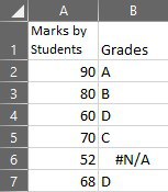
If we had used the formula

=IFS(H2>450,"A",H2>400,"B",H2>350,"C",H2>300,"D",H2<300,)

The returned result would look like this:

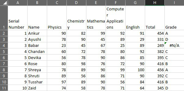
As the condition in cell I4 does not turn out to be true, and we had assigned no other value for this situation, it returns “#N/A.”

Example 2

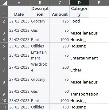
Assume you have a table of expenses and wish to categorize them based on their amount.

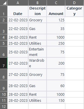
Our large table consists of the user’s expenses: the date, description, amount, and category. Here the category is unknown, and we must categorize the data according to its description and the amount spent.

Here the formula used will be:

=IFS(AND(B2="Groceries",C2>100), "Food", AND(B2="Groceries",C2<=100), "Miscellaneous", AND(B2="Gas",C2>50), "Transportation", AND(B2="Gas",C2<=50), "Miscellaneous", B2="Rent", "Housing", B2="Utilities", "Housing", B2="Entertainment", "Entertainment", B2="Shopping", "Shopping", TRUE, "Other")

This is comparable to the Else component of the If Else statement, which is used to avoid receiving the #N/A error in Excel.

After inputting the formula, the sheet will yield the following output:

IFS vs. SWITCH function

Excel's IF and SWITCH functions assess multiple conditions and return a value based on the first true condition. Yet, some significant distinctions between the two functions make them more appropriate for various scenarios.

The IFs function can run multiple conditions and return a value for the first true condition.

Each condition is checked until one is evaluated to be true. The value evaluated to be TRUE is returned. It returns either a blank space or '#N/A' if none of the values are true.

Here's an example:

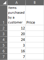
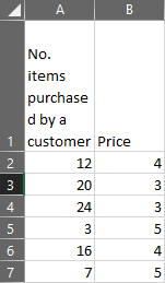
Imagine a store has different pricing tiers for how many things are purchased. If a consumer buys less than 10 products, the price per item is $5. If they buy less than 20 products, the price per item is $4.

If customers purchase further after purchasing 20 products, the price per item is $3

 The formula would be:

=IFS(A2<10,5,A2<20,4,A2>=20,3)

A2 reflects the number of products purchased in this scenario.

The function returns 5 if A2 is less than or equal to 10. The function returns 4 if A2 is between 11 and 20. If A2 exceeds 20, the method yields 3.

The SWITCH function, on the other hand, lets you examine an unmarried expression to a set of values and return the result that matches the first. The syntax is

=SWITCH(expression, value1, result1, [default or value2, result2],…[default or value3, result3])

The expression is evaluated in order against each value until a match is obtained. Then, the value of the corresponding result is returned. A default value might be returned as an option if no match is detected.

Here's an example of how to utilize the SWITCH function:

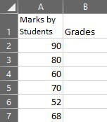
Imagine a teacher who wants to offer letter grades to students based on their numerical grades. For example, the following is the grading scale:

If the rating is between 90-100, one may be allotted an 'A,' if the score ranges from 80-89, one's grade will be 'B,' or if it's between 70-79, the grade is probably 'C,' if it's between 60-69, one may be allocated 'D,' and much less than 60 can be equal to an 'F.'

The formula used:

=SWITCH(TRUE,A2>=90,"A",A2>=80,"B",A2>=70,"C",A2>=60,"D",TRUE,"F")

A2 symbolizes the student's numerical grade in this scenario. First, the expression ">=90" is evaluated. Then, the function returns "A" if A2 is larger than or equal to 90. If this is not the case, the following expression, ">=80," is evaluated.

The process runs on a loop until a match is found or the default value gets returned.

When there are several conditions, the SWITCH function may be easier to read and manage than the other function. It also lets you utilize comparison operators in your expressions, which makes the formula more versatile.

The SWITCH function, on the other hand, has some limits. For example, it can only compare one expression to several values, whereas the IFs function can compare many conditions.

It also necessitates sorting the values in ascending order, which might be difficult. If the values cannot be easily sorted, it becomes difficult.

The IFs function performs better when testing several conditions. However, the SWITCH function performs better when evaluating a single expression against multiple values.

Conclusion

Excel's IFS function provides a major improvement in data analysis capabilities. It gives users a streamlined and effective way to handle intricate decision-making procedures.

IFS eliminates the need for nested IF statements by evaluating numerous conditions and returning the corresponding value based on the first true condition. This makes managing a variety of criteria more flexible and user-friendly.

It is an indispensable tool for activities like grading, data categorization, and sophisticated judgment due to its simple syntax and ability to evaluate up to 127 conditions.

The IFS function enables Excel users to gain deeper insights from their data and confidently make better-informed decisions by streamlining the procedures involved in data analysis and decision-making.

Free Resources

To continue learning and advancing your career, check out these additional helpful WSO resources:

• CRITBINOM Function
• IFERROR Function
• INFO Function
• MATCH Function
• RANK Function